Morris eSU (Sampling Uniformity) Global Sensitivity Toolbox

There are two Elementary Effects (EE) packages that complement the analysis: a) EE Sampling - to obtain the Morris samples based on a number of methods, including Sampling for Uniformity (SU); and b) EE Measures and Plots - after running the model with the EE samples it post-processes the results and provides Morris statistics and plots.

Download the Matlab code, sample inputs and documentation for the packages from the links below:

Please click on the tabs below to see the documentation for each of the packages.

EE Sampling |
EE Measures and Plots

Elementary Effects (EE) Sampling Package

Description

EE_Sampler_Mapper Package is a set of MATLAB functions that generates input factor samples for the method of Elementary Effects or Morris method (Morris, 1991). The main function to run is ‘Fac_Sampler.m’ (or its simplified command line form sampler.m). It generates input factor samples in a unit hyperspace and then transforms them according to the specified input probability distributions. Currently this tool gives five options for sampling strategy: (a) the method of Optimized Trajectories [OT] (Campolongo et al. 2007); (b) the Modified Optimized Trajectories [MOT] (Ruano et al., 2012); (c) Sampling for Uniformity [SU] (Khare et al., 2015); and (d) Enhanced Sampling for Uniformity [eSU] (Chitale et al., 2017); and (e) RadialeSU/ReSU (Chitale et al.) (in preparation).

Program Usage & Outputs

Syntax
Fac_Sampler(‘facfile’, ‘SS’, OvrSamSiz, NumLev, NumTraj, ‘SamFileType’)

A command line shell (sampler.m) is provided for those interested in compiling the program for use in mixed environments (i.e. unix scripts and others). The program can be compiled in the Matlab environment with 'mcc -m sampler.m'. This will produce a command line executable that can be run outside Matlab, or in another machine command line environment provided that the same runtime library version as the compiler is installed in the client machine (see Matlab Compiler Runtime download and instructions here). An example of use for this tool (inside and outside Matlab) would be:

sampler ‘try.fac’ ‘eSU’ 1 8 16 ‘Text’

Inputs:

(1) facfile: This is an ASCII '.fac' file that that follows the format (and can be generated) from SimLab v2.2.1 (Saltelli et al. 2004). For exact file formatting and distribution characteristics please refer SimLab v2.2 manual App. C (available here) (Saltelli et al. 2004). The file contains the following information:

(a) number of input factors (NumFact)

(b) default distribution truncation values

(2) SS: Sampling Strategy. Currently we provide five options:

(a) ‘OT’ - Campolongo et al. (2007) - Method of Optimized Trajectories

(b) ‘MOT’ - Ruano et al. (2012) - Method of Modified Optimized Trajectories

(d) ‘eSU’ - Chitale et al. (2017) – Enhanced Sampling for Uniformity

(e) ‘RadialeSU’ - Chitale et al. (in preparation) – Radial eSU

(3) OvrSamSize: Oversampling Size.

For OT and MOT the recommended oversampling size is 500-1000. For SU recommended oversampling size is 300. For eSU oversampling is not necessary i.e. we recommend OvrSamSize = 1. The current version of this EE_SamplerMapper tool interactively guides user to choose appropriate Oversampling size based on literature recommendations.

(4) NumLev: Number of input factor levels

In EE literature various values for number of levels have been suggested. However, the standard practice is to use even number of levels usually 4, 6 or 8. For SU/eSU and RadialeSU user can choose from NumLev = {4,6,8,10,12,14,16}. If user specifies NumLev that does not belong to this set, then it will be set to 4 by default.

(5) NumTraj: Number of trajectories to be generated

In EE literature recommended value for number of trajectories vary from as little as 2 to as large as 100. However, a number of studies have reported that 10-20 trajectories are sufficient. Chitale et al. (2017) indicates that for eSU the number of trajectories should be multiple of the number of levels to get better results. The current version of this EE_SamplerMapper tool interactively guides user to change/select number of trajectories whenever necessary. Presence of factor/s with ‘Nominal’ type of distribution needs further consideration while selecting NumTraj. This tool guides the user in adjusting NumTraj in such cases.

(6) SamFileType: Sample File Format. Currently we provide two options:

(a) ‘Excel’

(b) ‘Text’ (comma separated file with .sam extension)

Outputs:

(1) Factor_Sample: Input factor sample [ncol,nrows], where ncol = NumFact and nrows = NumTraj*(NumFact+1). Each column corresponds to one input factor

(2) *_FacSample.xlsx or *_FacSample.sam:

If user sets SamFileType = ‘Excel’ then Factor samples are written to an excel file ‘*_FacSample.xlsx’, where * i.e. first part of the file name is same as the first part of the ‘.fac’ file. (e.g. Factor sample for the input file ‘Example.fac’ will be saved in ‘Example_FacSample.xlsx’). If user sets SamFileType = ‘Text’ then Factor samples are written to a text file ‘*_FacSample.sam’, where * (i.e. first part of the file name) is the same as the first part of the ‘.fac’ file. In both types of files each column corresponds to a factor. Factor name is specified on the first row

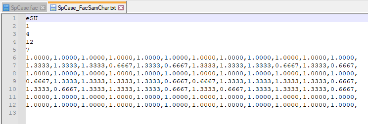
(3) *_FacSamChar.txt: Characteristics used for generating the sample are written to a text file ‘*_FacSamChar.txt’, where * i.e. first part of the file name is same as the first part of the ‘.fac’ file. (e.g. FacSamChar file for the input file ‘Example.fac’ will be saved as ‘Example_FacSamChar.txt’). Details of *_FacSamChar.txt file are as follows

First Line: Sampling Strategy – OT, MOT, SU, eSU or RadialeSU

Second Line: Oversampling Size

Third Line: Number of levels

Fourth Line: Number of trajectories

Fifth Line: Number of factors

Remaining Lines: Elementary Effects multiplication matrix, arranged by factors in rows and trajectories in columns. This matrix is useful for the cases when model has a Uniform Discrete factor/s with number categories different than NumLev.

Folder Structure:
There are 6 Matlab functions (i.e. m files) and five folders (Campolongo, Ruano, Khare, Enhanced_Khare, and Radial_Khare) included in this package (EE_Sampler_Mapper). Generated factor/input factor sample file *_FacSample.xlsx' or ‘*_FacSample.sam’ and ‘*_FacSamChar.txt’ will be stored in the folder same as ‘Fac_sampler.m’.

Input Factor Probability Distributions for facfile:
For the details about distribution characteristics please refer SimLab v2.2 user manual App A (available here) (Saltelli et al. 2004). Currently the following parameter distributions can be generated using this package:
(1) 'Uniform'
(2) 'LogUniform'
(3) 'Normal'
(4) 'LogNormal'
(5) Discrete (for categorical factors)

‘Nominal’ - uniform discrete for nominal factors

‘NUDiscrete’ – non-uniform discrete for nominal and ordinal factors

‘UDiscrete’ – uniform discrete for ordinal factors.

(6) 'Constant'
(7) 'Triangular'
(8) 'Weibull'
(9) 'Beta'
(10) 'Gamma'
(11) 'Exponential'
(12) 'Log10Uniform'

Note on Discrete Distributions. To make EE_SamplerMapper tool more flexible in its usage, we replaced the original Simlab (Saltelli et al. 2004) ‘Discrete’ distribution by the three types presented above (‘Nominal’, ‘NUDiscrete’, and ‘UDiscrete’).

(A) ‘Nominal’ uniform distribution for discrete nominal factors. A nominal variable (sometimes called a categorical variable) is one that has two or more categories, but there is no intrinsic ordering to the categories (for example “colors”, “gender”, etc.). For the ‘Nominal’ type factors it is necessary to ensure that all combinations of discrete levels are considered to get reliable EE based sensitivity measures. However, this increases the number of trajectories. Current version of the EE_SamplerMapper guides users to select appropriate number of trajectories i.e. NumTraj when it encounters the presence of ‘Nominal’ factors. Example: If modeler is to choose from a number of sub-models to be used to simulate a particular mechanism then that ‘sub-model’ is a factor for EE analysis with nominal discrete type of distribution. There is no restriction on number of discrete values/categories/options to be selected. However, larger the number of categories larger is the number of trajectories needed.

(B) ‘UDiscrete’ distributions are used for ordinal discrete factors with equiprobable categories. A discrete variable is ordinal when there is a clear ordering of the values, either numerical (i.e. $5, $10, $15) or non-numerical (i.e. "low, "medium" and "high"). An example of usage of this type of distribution would be the usage of application of EE sampling for design of experiments in ecotoxicology (Rodea-Palomares et al., 2016). Successful generation of sample for such a factor depends on number of categories used. If number of categories are not equal to the NumLev then it is not possible to get UDiscrete distribution due to mismatch between the two. In such cases instead of using NumLev defined by the user, this tool samples corresponding factor with NumLev = number of categories. Sampling is done with procedure consistent with the continuous distribution factors. However, this modification has implications on sensitivity indices calculations in such cases. The Elementary Effects multiplication matrix is calculated and used for this purpose. The multiplication factors are calculated as

If number of categories is even

If number of categories is odd

Where NC is the number of categories and Δx is x/[2(x-1)].

We have demonstrated this with an example (example 5) later in this manual.

(C) ‘NUDiscrete’ distributions can be used for ordinal discrete factors with non-uniform distributions. However, we want to warm users to be cautious about usage of this option. Accuracy of generated factor distributions depends on NumLev, number of categories, and corresponding weights/probability configuration assigned to such factor. E.g. for SU/eSU/RadialeSU if NumLev is 4, and factor has 3 categories, then only three non-uniform probability configurations can be generated for NUDiscrete factors without any issues for EE analysis – (1) {0.25, 0.5, 0.25}, (2) {0.5, 0.25, 0.25}, and (3) {0.25, 0.25, 0.5}. Note that if weights/probability configurations are not assigned properly this distribution can result in trajectories where NUDiscrete factors do not change values, and potentially result in inaccurate EE measures/ EE Screening. E.g. In case NumLev = 4 and there are two discrete categories with unequal probabilities, e.g. {0.25, 0.75} or {0.75, 0.25}, half of the trajectories will result in EEs being 0 and will result in inaccurate values of sensitivity measures. Hence, modelers should be careful while interpreting corresponding results. We strongly recommend checking if it is possible to generate a representative sample when NUDiscrete factor is present and potentially adjust NumLev and/or weights assigned to individual categories of NUDiscrete factor/s.

The use of the three discrete distributions is restricted to SU, eSU and RadialeSU. EE_Sampler_Mapper tool prompts user to choose appropriate sampling method when these types of distributions are present. We are currently expanding our tool to improve its utility in generation one more distribution – non-uniform nominal/NUNominal distribution. Please contact the authors for additional information if this feature is needed.

Probability distribution truncation

(A) When parameter distribution/distributions have long tails (Normal, LogNormal, Weibull, Gamma, Exponential), to get accurate results/ factor rankings consistent with variance-based SA methods (e.g. Sobol’), experience has shown that truncated distributions perform better. SimLab v2.2 truncates distributions at 12.5% and 87.5% i.e. overall 25% truncation. Though, ideal truncation may vary from model to model, we recommend 2.5% to 5% truncation from either side.

(B) If the user wants to use different truncations for different factors/parameters lower and upper percentiles (expressed as fractions) should be edited in the .fac' (please refer to App. C of SimLab v2.2 manualSimLab v2.2 manual App. C available here) (Saltelli et al. 2004). By default SimLab v2.2 sets these values these values at 0.001 and 0.999. See Example 2 in the following sections for additional details.

Examples

Example 1

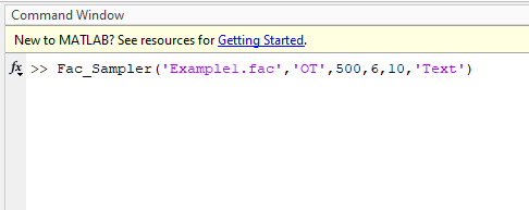
Generate 10 trajectory samples for factor file ‘Example1.fac’ (see package distribution) with OT method. Use oversampling size of 500 and 6 factor levels. Save outputs in text format (Example1_FacSample.sam). Type following in the Matlab Command window making sure that you are in EE_Sampler_Mapper folder.

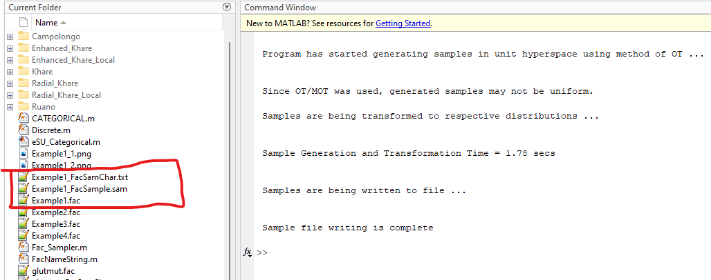
Output (notice new files Example1_FacSamChar.txt and Example1_FacSampler.sam on the left column)

Example 2

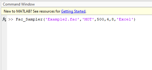
Generate samples for factors in ‘Example2.fac’ (see package distribution) using method of MOT. Generate 8 trajectories with 500 oversampling size, NumLev = 4. Save sample in excel format. Note that Example2.fac contains ‘Nominal’ and ‘UDiscrete’ type factors.Type following in Matlab command window.

Output:

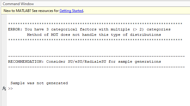
As expected, the sample was not generated and a warning is shown

Following the warning, we now generate the samples using eSU instead of MOT. Keep all other settings the same, except OverSamSiz = 1.

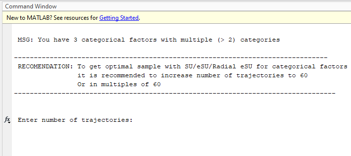
In this case, due to the presence of Nominal and UDiscrete factors, user was asked to increase number of trajectories as shown. Let’s increase number of trajectories to 60.

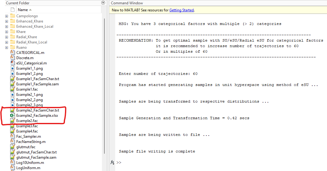
Example 3

Generate samples for factors in ‘Example3.fac’ (see package distribution) using method of eSU. Generate 10 trajectories with 100 oversampling size, NumLev = 10. Save sample in text format. Type following in Matlab command window.

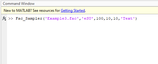
Output

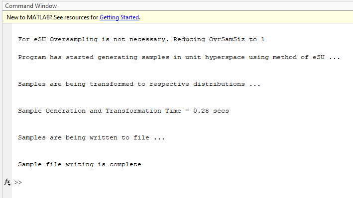
Let’s try generating sample for Example3.fac file with eSU. Try NumLev = 12, NumTraj = 8, OvrSamSiz = 1. Below are input and output screenshots

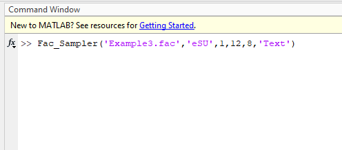
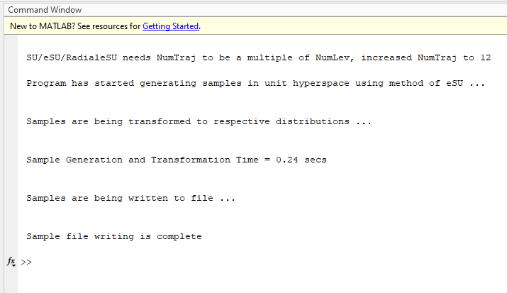
Since NumTraj = 8 is less than NumLev = 12, NumTraj will be increased to 12 to ensure uniformity of generated sample.

Output

Example 4

Generate samples for factors in ‘Example4.fac’ (see package distribution) using method of RadialeSU. Generate 15 trajectories with 1 oversampling size, NumLev = 12. Save sample in text format. Type following in Matlab command window.

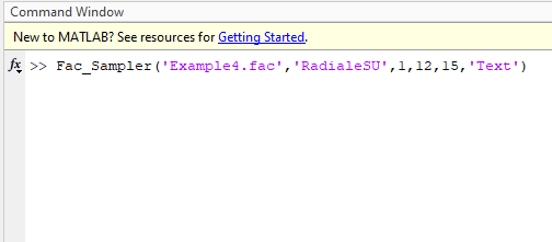
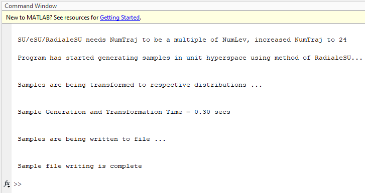
Since NumTraj is not multiple of NumLev, NumTraj will be increased to 24 (12x2)

Output

Example 5: Special Case 1 - UDiscrete factors with 3 categories and NumLev = 4

As discussed earlier, in the presence of discrete type of factors user needs to take cautious approach while generating sample for Elementary Effects analysis. One of such case is when we have one or more ordinal type discrete factors with 3 equiprobable categories (UDiscrete). This is a common situation in our experience. Also, using NumLev = 4 is also common and a common EE sample generation characteristic.

We have included an example ‘SpCase.fac’ file with 7 factors with this package. Among 7 factors p1 and p3 are UDiscrete and have 4 categories with (0.25, 0.25, 0.25, 0.25) configuration; p2, p4, and p5 are UDiscrete and have 3 categories with (0.3333, 0.3334, 0.3333) configuration; while p6 has Uniform distribution and p7 has 3 category Nominal distribution. For complete factor value details please see the actual SpCase.fac file.

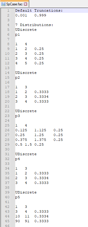
When this tool encounters the situation of factor/s with UDiscrete distribution, but NumLev not being multiple of number of discrete categories, it samples those factors with Number of Categories as NumLev and calculates Elementary Effects multiplication matrix as explained earlier. EE adjustment matrix is used by Sensitivity Measures tool to multiply raw elementary effects.

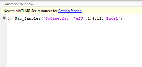
To generate sample for this ‘SpCase.fac’ use, SS = ‘eSU’, OvrSamSiz = 1, NumLev = 4, NumTraj = 12, and ‘Excel’ output format

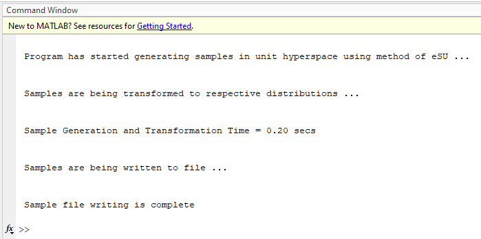
Outputs

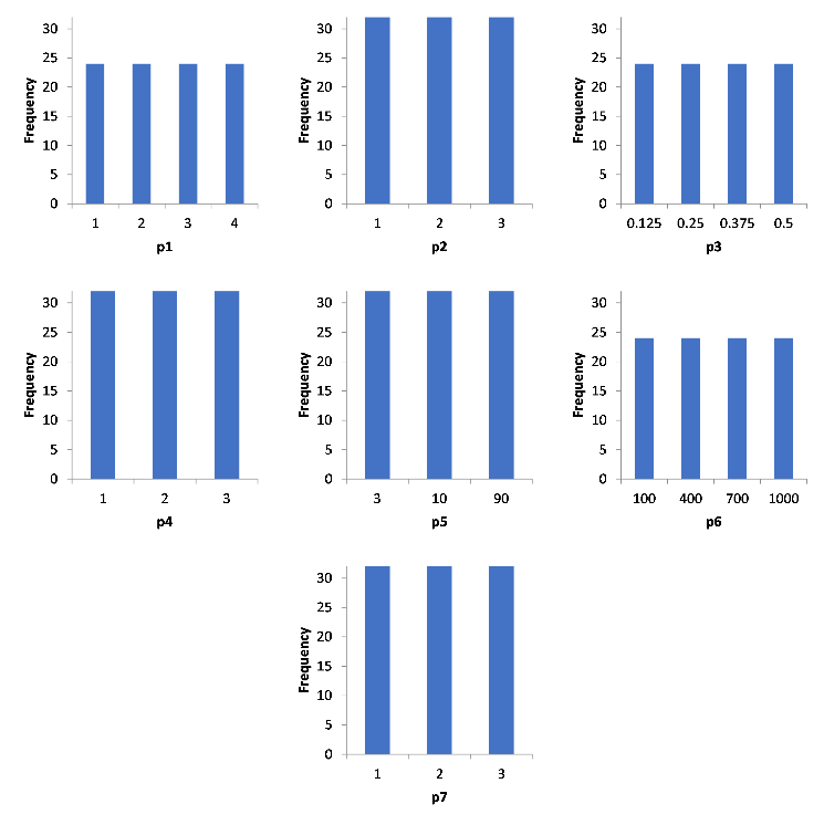
It can be observed that all factors have desired distributions

We can observe that p2, p4, and p5 (UDiscrete factors with 3 categories) have several EE multiplications values of calculated based on formulas presented earlier.

References

· Campolongo, F., Cariboni, J., Saltelli, A., 2007. An effective screening design for sensitivity analysis of large models. Environ. Model. Softw. 22, 1509e1518. http://dx.doi.org/10.1016/j.envsoft.2006.10.004.

· Chitale, J., Khare, Y.P., Muñoz-Carpena, R., Dulikravich, G.S., & Martinez, C.J., (2017) An effective parameter screening strategy for high dimensional models. ASME International Mechanical Engineering Congress and Exposition, Volume 7: Fluids Engineering ():V007T09A017. doi:10.1115/IMECE2017-71458.

· Khare, Y.P.*, Muñoz-Carpena, R., Rooney, R.W., Martinez, C.J. A multi-criteria trajectory-based parameter sampling strategy for the screening method of elementary effects. Environmental Modelling & Software 64:230-239. doi:10.1016/j.envsoft.2014.11.013.

· Khare, Y.P.*, C. Martinez, R. Muñoz-Carpena, A. Bottcher and A. James. 2019. Effective global sensitivity analysis for high-dimensional hydrologic and water quality models. ASCE Journal of Hydrologic Engineering 24(1):04018057. doi:10.1061/(ASCE)HE.1943-5584.0001726.

· Morris, M.D., 1991. Factorial sampling plans for preliminary computational exper- iments. Technometrics 33 (2), 161e174.

· Ruano, M.V., Ribes, J., Seco, A., Ferrer, J., 2012. An improved sampling strategy based on trajectory design for application of the Morris method to systems with many input factors. Environ. Model. Softw. 37, 103e109. http://dx.doi.org/10.1016/ j.envsoft.2012.03.008.

· Saltelli, A., S. Tarantola, F. Campolongo, and M. Ratto. 2004. Sensitivity Analysis in Practice: A Guide to Assessing Scientific Models. Chichester, U.K.: John Wiley and Sons. [with software SIMLAB v2.2.1 available here]

Program License

These Matlab (R) packages were developed by Drs. Yogesh Khare and Rafael Muñoz-Carpena. This program is distributed as Freeware/Public Domain under the terms of GNU-License. If the program is found useful, the authors ask that acknowledgment is given to its use in any resulting publication and the authors notified. The source code is available from the authors upon request.

We highly encourage using these packages for EE (Morris) sampling and sensitivity measures calculations with the eSU ('enhanced Sampling for Uniformity') method. If you use this package, kindly acknowledge our effort. Also, if you have any question in usage of this package, please contact us on the email address below.

· Yogesh Khare and Rafael Muñoz-Carpena
Agricultural & Biological Engineering
University of Florida
P.O. Box 110570
Frazier Rogers Hall
Gainesville, FL 32611-0570

(352) 392-1864
(352) 392-4092 (fax)
khareyogesh1@gmail.com, carpena@ufl.edu

Return to top

This page was last updated on March 29, 2024.