Morris eSU (Sampling Uniformity) Global Sensitivity Toolbox

There are two Elementary Effects (EE) packages that complement the analysis: a) EE Sampling - to obtain the Morris samples based on a number of methods, including Sampling for Uniformity (SU); and b) EE Measures and Plots - after running the model with the EE samples it post-processes the results and provides Morris statistics and plots.

Download the Matlab code, sample inputs and documentation for the packages from the links below:

Please click on the tabs below to see the documentation for each of the packages.

EE Sampling |
EE Measures and Plots

Elementary Effects (EE) Measures and Plots Package

Description

EE_SensitivityMeasures_Package is a set of Matlab functions that calculates sensitivity measures for the method of Elementary Effects/Morris method (Morris, 1991). Function ‘EE_SenMea_Calc.m’ is the main function that user needs to call from MATLAB command line. Calculated measures include modified sensitivity measures - μ* and σ based on (Campolongo et al. 2007) and original measure μ proposed by Morris (1991), and additions by the SU authors (Khare et al., 2015; Chitale et al., 2017).

Program Usage & Outputs

Syntax
EE_SenMea_Calc(FacFile,Fac_Sam_File,Fac_Sam_Char,Mod_Out_File,Per_Fac_Label)

Inputs:

(1) FacFile: This is an ASCII input factor '.fac' file that follows the format (and can be generated) from SimLab v2.2. For exact file formatting and distribution characteristics please refer SimLab v2.2 manual App. C (available here). Please see also the EE Sampling section for additional details pertaining the modifications introduced for Discrete distributions.

(2) Fac_Sam_File: This is an Excel(R)'*.xlsx' or ‘*.sam’ file (a comma separated text file) containing factor/parameter samples. This file is generated by the EE Sampling package.

(3) Fac_Sam_Char: This file is generated along with ‘*.xlsx’ file or ‘*.sam by Factor_Sampler_Mapper package for factor sample generation. This is a '*.txt' file which contains following information:

(a) Sampling Strategy (line 1)

(b) Over Sampling Size (line 2)

(d) Number of trajectories (line 4)

(e) Number of factors (line 5)

(f) Elementary Effects multiplication matrix (line 6 onwards)

(4) Mod_Out_File: This is a '*.xlsx' file or ASCII text file with ‘.out’, ‘.dat’ or ‘.txt’ extensions. This tool can handle both scalar and time series outputs. The specific formats are as follows.

Scalar Outputs

If the model output/s of interest are scalar then arrange them column-wise (tab, space or comma delimited for text files). Output names should be specified in the first row.

Time Series Outputs

If the model output of interest are timeseries, the file format is as follows. The file name needs to start with ‘Time’, e.g. ‘Time_DummyModOut.out’. Note that only one output can be included in one file

Excel

ASCII File

For timeseries outputs saved in ASCII files, format is similar to Excel file. Columns can be tab, comma or space separated and the file extension could be any of ‘.out’, ‘.txt’, ‘.dat’.

(5) Per_Fac_Label: Percentage of factors to be labeled in EE Plots. Typically, relatively few factors are well separated from origin and are of interest, we suggest labeling top 20% to 40% of factors based on µ* values (i.e. use 20 or 40 on this input).

Outputs:

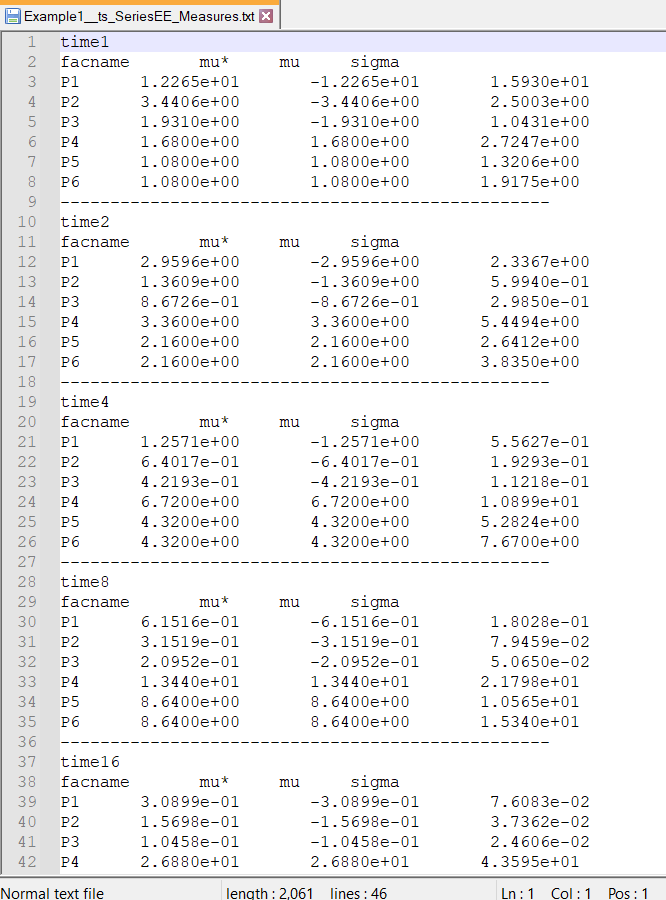
(1) EE_SA_Measures.txt: Sensitivity measures based on the method of Elementary Effects/ Morris method are saved in this text file, for each model output. In case timeseries outputs, calculated measures are reported for each time.

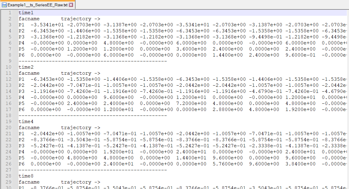
(2) Raw_EE.txt: This text file saves raw EEs for all outputs. For a given output, rows correspond to model factors while columns represent trajectories. These results can be used to verify accuracy of EEs or to perform any other analysis on Raw EEs as desired by the user.

(3) Raw_EE.mat: Information in this file is same as Raw_EE.txt, but is saved in ‘.mat’ (Matlab) format for users with Matlab proficiency.

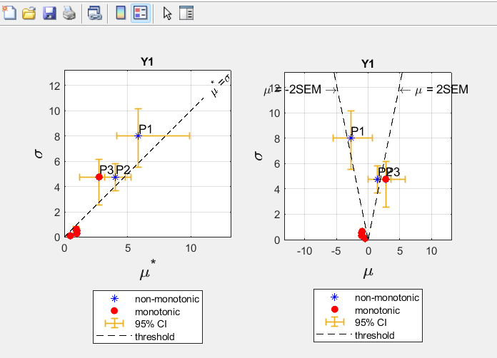
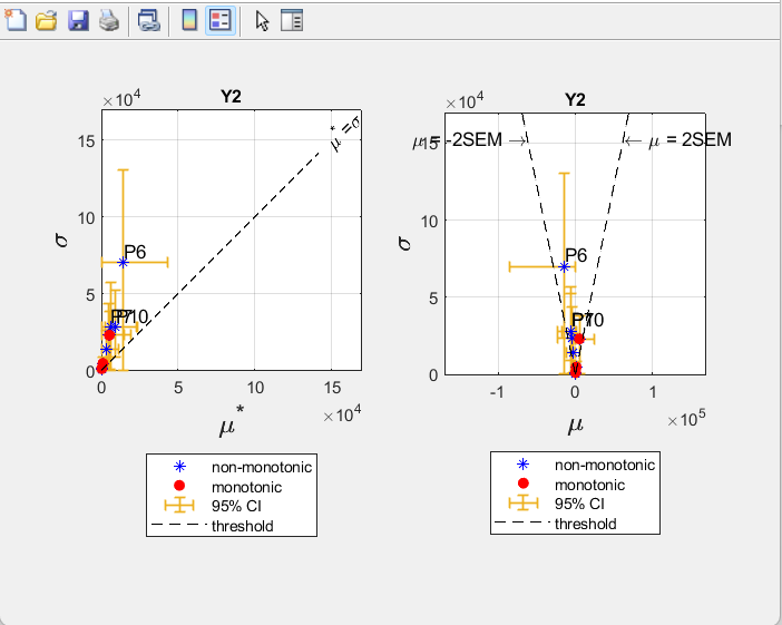
(4) Plots: Two figures/subplots are produced for each model output. The first subplot is a plot of μ* vs σ while the second one consists of μ vs σ. Additionally, we plot μ* = σ line (dotted black line) on the first sub-plot and μ = -/+ 2 σ/(√r) lines (solid black line, with r number of sampling trajectories) on the second subplot. Factors above the lines in both plots are considered to have dominant interactions effects. The µ = -/+2 σ/(√r) lines were proposed by Morris (1991) to identify factors with dominant non-additive/non-linear effects. The 1:1 line (i.e. µ*=σ) threshold is based on Chu-Agor et al. (2011) and Khare et al. (2019). Additionally, factors for which µ* = |µ| holds true, i.e. factors with perfectly monotonic effects, are indicated by solid red circles while rest are indicated by blue asterisk. Also, bootstrapping based 95% CI for µ*, µ, and σ are indicated (golden color) on the subplots by horizontal error bars. Plots are automatically saved as PDF and JPG files. In case of timeseries outputs, a figure with three subplots (µ* vs time index, µ vs time index, and σ vs time index) is generated in PDF and JPG format.

Folder Structure:

This package consists of 7 Matlab functions (i.e. m files) namely (a) EE_SenMea_Calc, (b) EE_Plots, (c) Morris_Measure_Groups, (d) Morris_Measures, (e) Morris_Measure_Radial, (f) EE_Rad_Traj, and (g) ReadFacDist saved in folder ‘EE_SensitivityMeasures’. Output files – ‘EE_SA_Measures.txt’, ‘EE_Raw.txt’, ‘EE_Raw.mat’, and plots (PDFs and JPGs) will be saved in the package folder.

For demonstration purposes we have provided input files required for each of the examples presented in this documentation. Please note that if users generate their own samples with the EE Sampling package for these examples, they should also recalculate the example model outputs as the EE measures would differ from the ones presented below.

Examples of syntax:

(a) If both sample and model output files are excel (.xlsx) files.

EE_SenMea_Calc(‘Example_FacFile.fac’, 'Example_Sample.xlsx', 'Example_SampleChar.txt', 'Example_Output.xlsx', 20)

(b) If sample file is *.sam and model output file is *.out

EE_SenMea_Calc(‘Example_FacFile.fac’, 'Example_Sample.sam', 'Example_SampleChar.txt', 'Example_Output.out', 20)

EE_SenMea_Calc(‘Example_FacFile.fac’, 'Example_Sample.sam', 'Example_SampleChar.txt', 'Example_Output.xlsx', 20)

(d) If sample file is *.xlsx and model output file is *.dat

EE_SenMea_Calc(‘Example_FacFile.fac’, 'Example_Sample.xlsx', 'Example_SampleChar.txt', 'Example_Output.dat’, 20)

Input/Output Example

Example 1

This is based on Example1 sample generated in the EE_Sampling package documentation.

Model output:

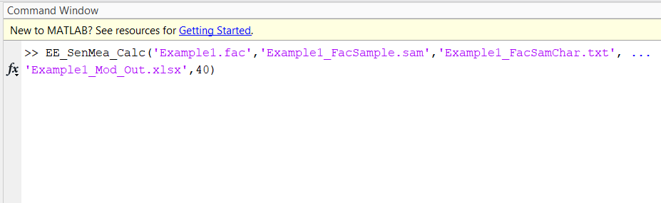
Model outputs results were saved in ‘Example1_Mod_Out.xlsx’ file. To calculate EE measures, first copy previously generated ‘Example1_FacSample.sam’ and ‘Example1_FacSamChar.txt’ files to EE_SensitivityMeasures Package. Then type the following in Matlab command window (make sure that EE_SensitivityMeasures Package is the active Matlab folder):

This will generate the figure below, which is automatically saved as a PDF file. EE sensitivity indices (µ*, µ and σ) are also written to ‘Example1_EE_Measures.txt’. Both files are saved in EE_SensitivityMeasures_Package directory.

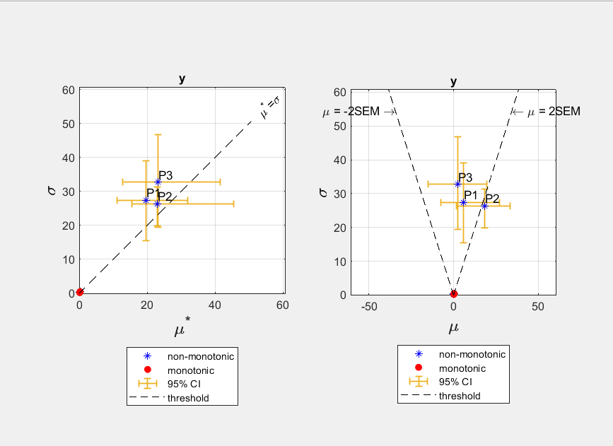
Note that we specified to label top 40% of the factors. In this case there are 6 model factors and hence after rounding up (6*0.4 = 2.4 -> 3) top three factors were labeled.

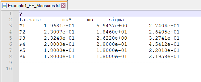
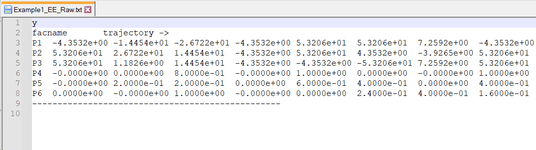
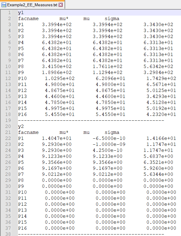
The two screenshots above show the EE_Measures.txt and EE_Raw.txt ASCII text files produced by the package that summarize the EE measures.

Example 2

This is based on Example 2 sampling generated in the EE Sampling package documentation.

Model output:

Model outputs results were saved in ‘Example2_Mod_Output.txt’ file (tab delimited). To calculate EE measures, first copy previously generated ‘Example2_FacSample.xlsx’ and ‘Example2_FacSamChar.txt’ files to the 'EE_SensitivityMeasures_Package' directory. Then type following in Matlab command window (make sure that EE_SensitivityMeasures_Package is the active Matlab folder):

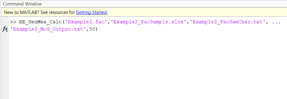
Output:

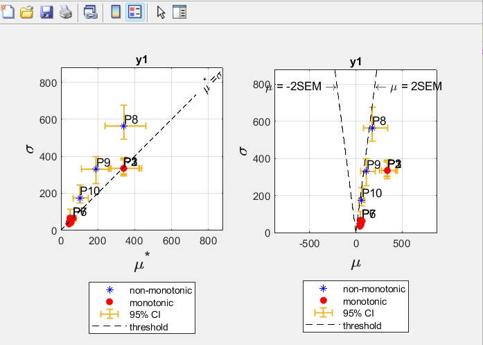
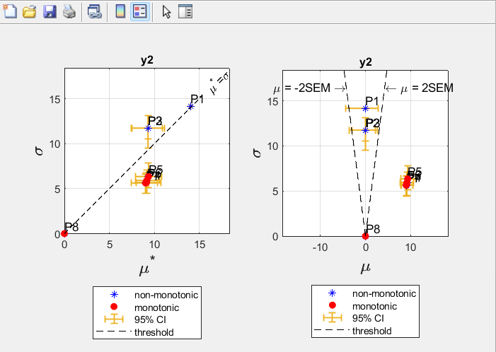
Note: The sample for this example was generated with the eSU method. For the second output (y2), it was expected that (1) P8 to P16 will have zero sensitivity indices, (2) P2 and P3 should have identical sensitivity indices due to their distributions and nature of output function, (3) P4 to P7 should have identical indices, and (4) P1, P2 and P3 would be non-monotonic. From the calculated indices three of these four things were found to be true. Though sensitivity measures for P4 to P7 were not identical they were relatively close.

To import Raw EEs for this example, type “load Example2_EERaw.mat” in the Matlab command window, which will load EERaw in Matlab Workspace as shown below,

Example 3

This is based on Example 3 sample generated in the EE Sampling package documentation (please see details following the link on top of this page).

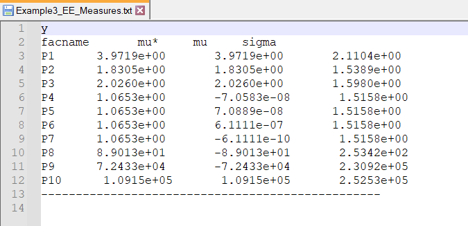
Model Output: y= P₁*(P₄+P₅) + P₂P₆ +P₃P₇ + [P₁₀/(P₈+P₉)]

Model outputs results were saved in ‘Example3_Mod_Out.out’ file. To calculate EE measures, first copy previously generated ‘Example3_FacSample.sam’ and ‘Example3_FacSamChar.txt’ files to the 'EE_SensitivityMeasures_Package' directory. Then type the following in Matlab command window (make sure that EE_SensitivityMeasures_Package is the active Matlab folder):

Package will produce following figure, which is automatically saved as PDF and JPG files. EE sensitivity indices (Mu*, mu and sigma) are also written to ‘Example3_EE_Measures.txt’. Both files are saved in EE_SensitivityMeasures package along with Example3_EERaw.mat and Example3_EERaw.txt.

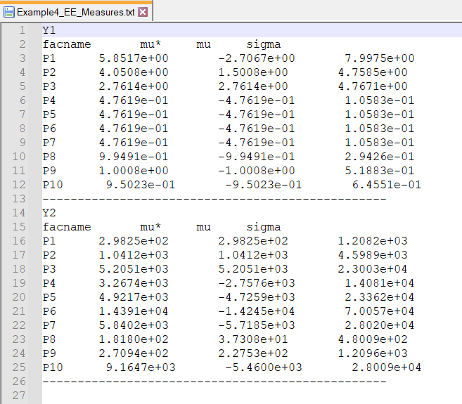
Example 4

This is based on Example 4 sample generated based o3n ‘RadialeSU’ method in the EE Sampling package documentation.

Model Outputs:

The model outputs results were saved in ‘Example4_Mod_Out.dat’ file (a comma separated ASCII file). To calculate EE measures, first copy previously generated ‘Example4_FacSample.sam’ and ‘Example4_FacSamChar.txt’ files to EE_SensitivityMeasures_Package directory. Then type the following in Matlab command window (make sure that EE_SensitivityMeasures Package is the active Matlab folder):

With output:

Example 5: Special case of constant model inputs

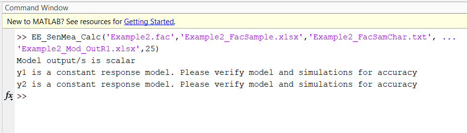
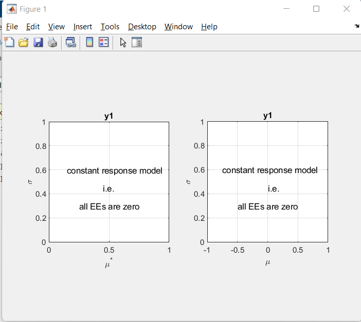
Sometimes the model output does not change due to multiple reasons including (a) the model is not a function of the factors that are being varied, (b) the output is a constant, (c) simulation errors. In such a case all Elementary Effects and hence sensitivity measures will be zero and the tool will issue a warning on the Matlab command window and plots.
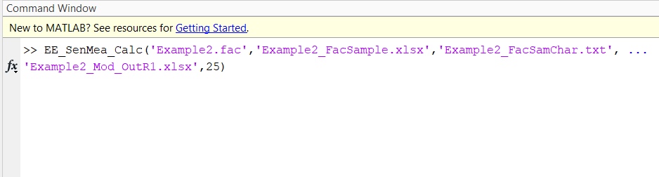
To demonstrate this, we have modified Example 2 (presented earlier). The new model outputs are constants, y₁ = 0 and y₂= 3. The new outputs were saved in ‘Example2_Mod_OutR1.xlsx’. Please see the following figures for details,

With output:

Example 6: Special Case – Udiscrete Factors

This is based on Special Case sample generated based on ‘eSU’ method in the EE Sampling package documentation. In this example we have several factors with UDiscrete distributions for which number of categories were not equal to NumLev = 4 that was defined to generate the factor sample.

Model Outputs:

As shown in the Sampler Mapper tool documentation, for P2, P4, and P5 Elementary Effects multiplication matrix has values different from 1. The model outputs results were saved in ‘SpCase_Mod_Out.xlsx’ file. To calculate EE measures, first copy previously generated ‘SpCase_FacSample.xlsx’ and ‘SpCase_FacSamChar.txt’ files to EE_SensitivityMeasures_Package directory. Then type the following in Matlab command window (make sure that EE_SensitivityMeasures Package is the active Matlab folder):

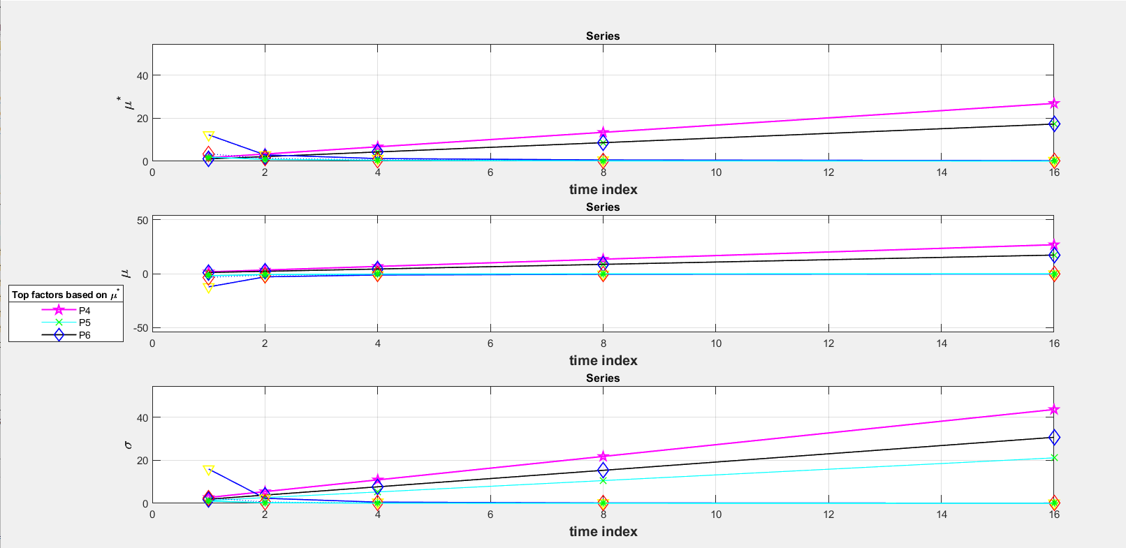
Example 7: Time Series Output

This timeseries output example is based on Example 1 sample generated in the EE Sampling package documentation. The model output is calculated using following function.

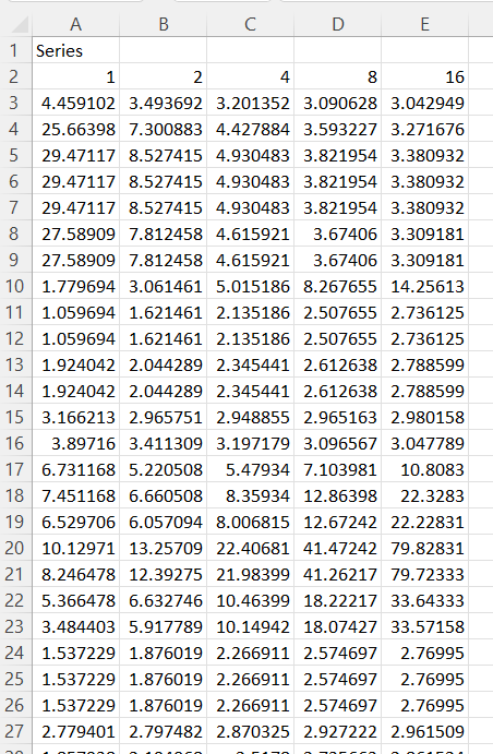
Model Outputs:

This model was evaluated for t = {1, 2, 4, 8, 16} and saved in an excel file ‘Time_Series_Out.xlsx’ as shown below. Please refer to the Syntax section of this documentation for time series output file format details. Note that timeseries output file name needs to start with ‘Time’.

To calculate sensitivity measures for this output type following in Matlab command window

The sensitivity measures timeseries outputs are as shown

Sensitivity Measures text outputs

Raw EE outputs

References

· Campolongo, F., Cariboni, J., Saltelli, A., 2007. An effective screening design for sensitivity analysis of large models. Environ. Model. Softw. 22, 1509e1518. http://dx.doi.org/10.1016/j.envsoft.2006.10.004.

· Chitale, J., Khare, Y.P., Muñoz-Carpena, R., Dulikravich, G.S., & Martinez, C.J., (2017) An effective parameter screening strategy for high dimensional models. ASME International Mechanical Engineering Congress and Exposition, Volume 7: Fluids Engineering ():V007T09A017. doi:10.1115/IMECE2017-71458.

· Khare, Y.P.*, Muñoz-Carpena, R., Rooney, R.W., Martinez, C.J. A multi-criteria trajectory-based parameter sampling strategy for the screening method of elementary effects. Environmental Modelling & Software 64:230-239. doi:10.1016/j.envsoft.2014.11.013.

· Khare, Y.P.*, C. Martinez, R. Muñoz-Carpena, A. Bottcher and A. James. 2019. Effective global sensitivity analysis for high-dimensional hydrologic and water quality models. ASCE Journal of Hydrologic Engineering 24(1):04018057. doi:10.1061/(ASCE)HE.1943-5584.0001726.

· Morris, M.D., 1991. Factorial sampling plans for preliminary computational exper- iments. Technometrics 33 (2), 161e174.

· Ruano, M.V., Ribes, J., Seco, A., Ferrer, J., 2012. An improved sampling strategy based on trajectory design for application of the Morris method to systems with many input factors. Environ. Model. Softw. 37, 103e109. http://dx.doi.org/10.1016/ j.envsoft.2012.03.008.

· Saltelli, A., S. Tarantola, F. Campolongo, and M. Ratto. 2004. Sensitivity Analysis in Practice: A Guide to Assessing Scientific Models. Chichester, U.K.: John Wiley and Sons. [with software SIMLAB v2.2.1 available here]

Program License

These Matlab (R) packages were developed by Drs. Yogesh Khare and Rafael Muñoz-Carpena. This program is distributed as Freeware/Public Domain under the terms of GNU-License. If the program is found useful, the authors ask that acknowledgment is given to its use in any resulting publication and the authors notified. The source code is available from the authors upon request.

We highly encourage using these packages for EE (Morris) sampling and sensitivity measures calculations with the eSU ('enhanced Sampling for Uniformity') method. If you use this package, kindly acknowledge our effort. Also, if you have any question in usage of this package, please contact us on the email address below.

· Yogesh Khare and Rafael Muñoz-Carpena
Agricultural & Biological Engineering
University of Florida
P.O. Box 110570
Frazier Rogers Hall
Gainesville, FL 32611-0570

(352) 392-1864
(352) 392-4092 (fax)
khareyogesh1@gmail.com, carpena@ufl.edu

Return to top

This page was last updated on March 29, 2024.